Index
- Introduction
- Ozone Sources
- Patterns of Ozone Concentrations and Exposure
- Effects on Plants
- Exposure Indices
- Literature Cited
Introduction
Ozone is a highly reactive form of oxygen. An ozone molecule is composed of three oxygen atoms (O3), instead of the two oxygen atoms in the molecular oxygen (O2) that we need in order to survive. In the upper atmosphere (stratosphere), the protective ozone layer is beneficial to people because it shields us from the harmful effects of ultra-violet radiation. However, ozone in the lower atmosphere (troposphere) is a powerful oxidizing agent that can damage human lung tissue and the tissue found in the leaves of plants. For more information about ozone’s effects on humans, refer to the EPA brochure Ozone and Your Health.
Ozone Sources
Ozone is formed in the lower atmosphere primarily by nitrogen oxides (NOx) reacting with volatile organic compounds (VOCs) on warm, sunny days. Nitrogen oxides are released into the atmosphere as a by-product of any combustion. For example, nitrogen oxides are released from the burning of vegetation during a fire. However, internal combustion engines (especially automobiles) and coal-fired power plants are the main sources of nitrogen oxides in the eastern United States. VOCs, or hydrocarbons, also come from man-made sources such as cars, service stations, dry cleaners, and factories and from natural sources such as trees and other vegetation. In fact, the main source of VOCs, in the southeastern United States, is from gases released by trees and other vegetation.

Patterns of Ozone Concentrations and Exposure
Ozone exposures are usually greatest close to large urban areas like Dallas, Texas; or Atlanta, Georgia. Ozone exposures are higher in these major cities because there are more cars, industry and other nitrogen oxide emissions sources then rural areas. Ozone concentrations can increase considerably on hot-sunny days when there is a stagnant air mass (i.e. little to no winds) present. Therefore, ozone is primarily a problem during the summer months, when heat and sunlight are more intense. Furthermore, the ozone formed in cities, or the nitrogen oxides originating in cities can be transported long distances into the rural areas. For example, in western North Carolina, the high elevations above 4000 feet have greater ozone exposures than nearby low-elevation areas. For example, the figure below shows the average ozone concentration for each hour of the day for a low elevation and a high elevation ozone-monitoring site. The low elevation site is adjacent to Asheville, North Carolina (called Bent Creek), and the high elevation site is near Shining Rock Wilderness. It is noteworthy that these two sites are about 15 miles apart, and separated by about 3000 feet in elevation.
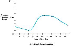
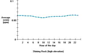
Average ozone concentrations for each hour of the day (April through October 1998) for a low elevation (top) and high elevation (bottom) sites. The low elevation site has a diurnal pattern in the ozone exposure and also shows that at lower elevations the ozone exposures are less than the ozone exposures found at high elevations. Results were produced using the Ozone Calculator.
The Bent Creek data shows a typical pattern (called a diurnal pattern) of ozone concentrations throughout the day (Berry, C.R., 1964). Ozone concentrations begin to rise in the morning and then decrease after the sun sets in the evening. Remember the recipe to form ozone is on warm sunny days, nitrogen oxides react with the VOCs. One pattern the Bent Creek data shows (right) is the ozone concentrations increase as the solar radiation and temperatures increase during the day. The Bent Creek data also reflects people’s daily activities. Typically, electrical generation (a major source of nitrogen oxides) increases in the morning as people get ready for work, and remains high on hot days in order to provide electricity to cool people’s homes and businesses. Also, when people drive to work each day they release nitrogen oxides from the tailpipes of their automobiles. The large amount of nitrogen oxides released early in the day contributes to recipe that forms ozone. The combination of a favorable environment and high nitrogen oxide emissions makes high ozone concentrations during the day.
Conversely, later in the day, many people drive home from work and electrical demand remains high on the hot days – thus there are still large amounts of nitrogen oxides released into the atmosphere. Solar radiation declines until sunset and the temperature also decreases. As nightfall approaches there is a lower likelihood that ozone will form because there is not enough sunlight (ultraviolet radiation) to cause the reactions necessary to form ozone. The nitrogen oxide emissions then serve an interesting role due to their abundance. Instead of contributing to ozone formation, the nitrogen oxides react with the ozone present in the atmosphere and cause a reduction of ozone concentrations during the nighttime. This occurs because nitrogen oxide molecules, in the absence of heat and strong sunlight, remove the third oxygen atom from the unstable ozone molecule.
In mountain valleys, such as occur near Bent Creek, ozone-forming pollution comes from both local and out-of-state sources. Winds can carry ozone formed in urban areas long distances to surrounding rural areas. Much of the ozone pollution at high elevations in the mountains of Western North Carolina is transported by winds from other states. The results from the high elevation ozone monitoring site near Shining Rock Wilderness (figure above) show ozone concentrations do not change throughout the day and that average concentrations are greater than at the Bent Creek site. Consequently, people and vegetation at higher elevations are exposed to more ozone then people and vegetation at low elevations.
Effect on Plants
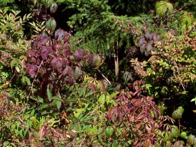 Ozone effects on plants are most pronounced when soil moisture and nutrients are adequate and ozone concentrations are high. Under good soil moisture and nutrient conditions the ozone will enter through openings into the leaf and damage the cells that produce the food for the plants. Once the ozone is absorbed into the leaf, some plants spend energy to produce bio-chemicals that can neutralize a toxic effect from the ozone. Other plants will suffer from a toxic effect, and growth loss and/or visible symptoms may occur. The presence of ozone in an area can be detected when consistent and known symptoms are observed on the upper-leaf surface of a sensitive plant species. For example, some air specialists use blackberry plants as a “bio-indicator” of ground level ozone. The photograph to the right shows the severe reddening of the blackberry foliage near Shining Rock Wilderness in western North Carolina when both adequate soil moisture and high ozone concentrations were present.
The presence of ozone symptoms is not an accurate indicator of how much growth loss has occurred to a sensitive plant from ozone exposure. Therefore, some air resource specialists rely upon measurements taken with ozone monitoring equipment in order to predict if growth loss has occurred. Ozone monitors provides over 4000 ozone readings from April through October. Researchers and technical specialists have examined ways to summarize and use this extensive information. The Ozone Calculator is one tool that has been developed to estimate if ozone exposures recorded at a monitoring site could cause a growth loss to the vegetation.
Exposure Indices
There are two important statistics used to estimate the growth loss to vegetation when summarizing data from an ozone monitor. The N100 statistic is the number of hours when the measured ozone concentration is greater than or equal to 0.100 parts per million (ppm). Experimental trials with a frequent number of peaks (hourly averages greater than or equal to 0.100 ppm) have been demonstrated to cause greater growth loss to vegetation than trials with no peaks in the exposure regime (Hogsett et al., 1985; Musselman et al., 1983; and Musselman et al., 1986). For this reason, the W126 (Lefohn and Runeckles, 1987) was developed as a biologically meaningful way to summarize hourly average ozone data. The W126 places a greater weight on the measured values as the concentrations increase. Thus, it is possible for a high W126 value to occur with few to no hours above 0.100 ppm. Therefore, it is also necessary to determine the number of hours the ozone concentrations are greater than or equal to 0.100 ppm. It should also be noted the lack of N100 values does not mean ozone symptoms will not be present when field surveys are conducted.
Ozone Exposure Indices for Vegetation
W126:
The W126 exposure index does not utilize a threshold value, but weights differentially all hourly average concentrations. Significant weighting greater than 0 occurs at all hourly average concentrations above 0.04 ppm. The use of a 0 weighting for hourly average concentrations less than 0.04 ppm was intentionally designed into the W126 so as to reflect near background levels. The W126 has weighting of approximately 1 for all hourly average concentrations equal to and above 0.100 ppm. The weighting of 1 at these concentrations was based on informal discussions with vegetation researchers in California whose vegetation experienced repeated occurrences of hourly values equal to and above 0.100 ppm. This was a subjective decision and it is recognized that every species will have a different weighting function.
N100:
The number of hourly average concentrations equal to or greater than 0.100 ppm.
Taken from A.S.L & Associates at: //www.asl-associates.com/example2.htm
Vegetation's sensitivity to ozone varies -- not only between species, but also within a species. For example, there may be two black cherry trees growing next to one another, and one will have severe ozone symptoms while the adjacent black cherry has no visible symptoms. An example of the variation between species can be seen when an analysis is conducted with Ozone Calculator. In 1998, Shining Rock Wilderness had a W126 value of 104.3227 and had 43 hours when the ozone concentration was greater than or equal to 0.100 ppm. Using these values as inputs, the estimated growth loss for one black cherry study was 26.1 percent, for red maple the growth loss was 5.6 percent, and for sugar maple the growth loss was estimated to be 0.1 percent. Assuming there were adequate nutrients and soil moisture, the predicted growth losses indicated that black cherry is more sensitive to ozone than red maple, which is more sensitive than sugar maple.
1998 Shining Rock
W126 = 104.3227, N100 = 43 hours
Growth Loss (%) |
|
Black Cherry |
26.1 |
Red Maple |
5.6 |
Sugar Maple |
0.1 |
Literature Cited
Berry, C.R. 1964. Differences in concentrations of surface oxident between valley and mountain conditions in the Southern Appalachians. JAPCA 15(6): 238-239.
Hogsett, W. E.; Plocher M; Wildman V.; Tingey, D. T. and Benett, J. P. 1985. Growth response of two varieties of slash pine seedlings to chronic ozone exposures. Can. J. Botany 63:2369-2376.
Lefohn, A. S.;Runeckles, V. C. 1987. Establishing a standard to protect vegetation - ozone exposure/dose considerations. Atmos. Environ. 21:561-568.
Musselman, R. C.; Oshima, R. J. and Gallavan, R. E. 1983. Significance of pollutant concentration distribution in the response of 'red kidney' beans to ozone. J. Am. Soc. Hort. Sci. 108:347-351.
Musselman, R. C.; Huerta, A. J.; McCool, P. M.; and Oshima, R. J. 1986. Response of beans to simulated ambient and uniform ozone distribution with equal peak concentrations. J. Am. Soc. Hort. Sci. 111:470-473.
updated: 3/21/13